reyemsaibot

SAP BI Blog about SAP BW/4HANA, Analysis for Office and SAP HANA - by Tobias Meyer

Blog

  • SAP Datasphere Hierarchies with unassigned nodes

    Unassigned nodes in BW query are a common case. This wasn’t available in SAP Datasphere for a long time and leads to some incorrect data while displaying the aggregated data in hierarchy form.


    There is also an influence request in the influence portal. SAP still hasn’t implemented yet a good soulation and the request is still open but there is a hint for a SAP online help entry how to
    solve the issue. The request is 304831.


    It is only available through the validation rules. The validation rules allow you to identify missing or enhanced hierarchy notes in your hierarchy. 


    The help entry is found under the name „Collect Unassigned Fact Records for Inclusion in Aggregations and Visualizations“. It has no link to the Hierarchy with Directoy entry nor is it
    linked with the Creating Analytic Model page. 


    With click on the validation of the fact view you get the information about missing hierarchy nodes in my GL Account hierarchy.

    Data Validation: Missing Hierarchy Nodes
    Data Validation: Missing Hierarchy Nodes

    Under „Details,“ you can find information on how to disable this behavior. 

    Missing Hierarchy Nodes: Detail
    Missing Hierarchy Nodes: Detail

    You can download the automatically created CSN files.  After importing them to your Datasphere tenant, you will see these three objects.

    Data Builder: Imported Objects
    Data Builder: Imported Objects

    Now we have to change the hierarchy association in the dimension to the enhanced object.
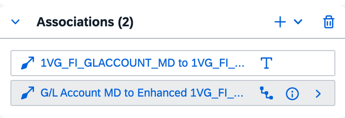
    Dimension Association
    Dimension Association

    Now you deploy the dimension and make the validation again. As you can see now there are no missing hierarchy nodes.
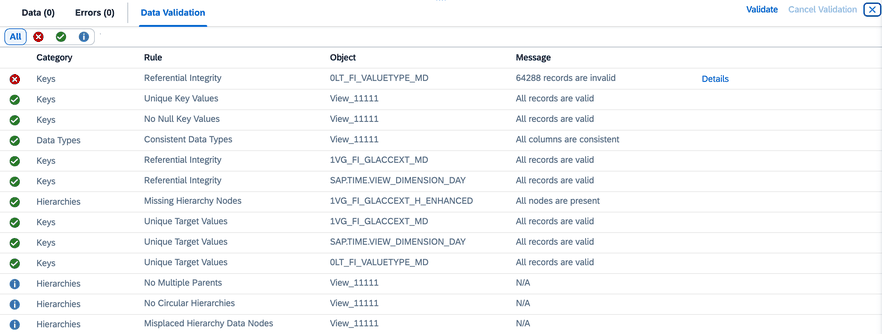
    Data Validation without issing hierachy nodes
    Data Validation without issing hierachy nodes

    The analytic model now correctly displays the unassigned nodes when I display the hierarchy.
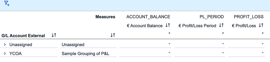
     

    Hierarchy in Analytic Model with unassigned nodes
    Hierarchy in Analytic Model with unassigned nodes

    Conclusion

    I don’t understand why SAP doesn’t do this automatically or why it’s hidden under the validation rules of a fact model. After completing the validation and changing the dimension association, the
    dimension can be used anywhere, and unassigned nodes will appear under „Unassigned Node.“


    I hope this information helps you correctly display unassigned nodes in the hierarchy.

    author.


    Hi,

    I am Tobias, I write this blog since 2014, you can find me on LinkedIn and
    YouTube. I work as a Data &
    Analytics Consultant. If you want, you can leave me a PayPal coffee donation.
    You can also contact me directly if you want.


  • SAP Inside Track Netherlands (sitNL)

    SAP Inside Track Netherlands @ SAP 's-Hertogenbosch
    SAP Inside Track Netherlands @ SAP ’s-Hertogenbosch

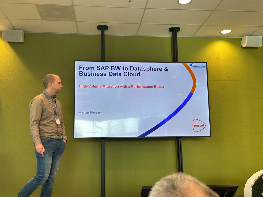
    Last weekend, I attended the SAP Inside Track Netherlands (sitNL) event at the Herzog Bosch Edison Community. Ronald and Tim were
    some of the organizers of this event, and I presented our customer project, „Road from BW 7.5 on AnyDB to Datasphere and Beyond.“ The 15th annual SAP Inside Track Netherlands has taken
    place. It was also a celebration featuring highlights from previous years.

    The agenda was quite interesting. There was a lot of AI stuff, as well as other presentations related to Datasphere.  The first one was about migrating high-volume BW to Datasphere, as well
    as the challenges they had to overcome. It was interesting to learn how many data records they have in this project and how they solved the issue of handling millions of records, tracking
    duplicates, and applying performance optimization. 

    The second presentation was all about learning about replication flows in Datasphere. The presentation covered best practices for using replication flows in a greenfield data project and what you
    can do with replication flows.


    In addition to the interesting presentations, there was a lot of good exchange of ideas.


    If you’re interested in my presentation, you can download it here. I hope to see many of you again next time. On the Inside Track Netherlands

    Conclusion

    I really like community events because you can learn a lot from them. There is also no competition between the different consulting firms. People like to share their knowledge, and you can have
    good conversations with them. 


    Sometimes, someone else writes a good article, and I’m happy when it solves my problem. If you have the time, attend these events and benefit from the knowledge. If you are ready, present your
    story. Hopefully, I will see you next time at sitNL!

    author.


    Hi,

    I am Tobias, I write this blog since 2014, you can find me on LinkedIn and
    YouTube. I work as a Data &
    Analytics Consultant. If you want, you can leave me a PayPal coffee donation.
    You can also contact me directly if you want.


  • Datasphere Customer Exit Variable Concept

    This blog post is all about customer exit variables. In SAP Business Warehouse, including BW/4HANA and BW on HANA, every customer has several. Now, it is time to bring this concept into SAP
    Datasphere.

    Familiarity with BW logic is assumed; it will not be explained in detail here.

    Some customers have implemented customer exit variables with different classes and tables to map something. For more information, see my old post about the concepts of customer exit variables in
    BW/4HANA.


    Now, back to SAP Datasphere. For a long time, Analytic Models has offered the possibility to consume variables as either Derived Variables or Dynamic Default.

    When compared to BW, the derived variables are similar to I_STEP 2 when the variable is
    not input-ready. Dynamic default variables are like I_STEP 1, which occurs before the variable prompt pops up.

    Sandy showed us in the Datasphere Topic Group how to achieve this. This is
    also documented in the SAP Community.

    https://community.sap.com/t5/technology-blog-posts-by-sap/sap-datasphere-bw-series-getting-started-part-2/ba-p/13953994


    I used this approach and enriched it with more time-based logic.

    • today
    • yesterday
    • last working day
    • same month last year
    • last year

    and many more. I think this is a good starting point for the time filtering you normally need. The code is always pretty much the same and looks like this:

    SELECT 'Yesterday' AS "Time_Description",
               ADD_DAYS(DATE_SQL, -1) as "Start_Date",
               ADD_DAYS(DATE_SQL, -1) as "Endt_Date",
               '' as "Date"
     FROM "SAP.TIME.VIEW_DIMENSION_DAY"
     WHERE "DATE_SQL" = CURRENT_DATE   
    

    I think everyone can adopt this. I won’t go into detail for each time option.


    In addition to time logic, you can also create customer exit variables for other dimensions.

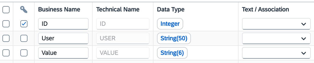
    Let me explain this approach in more detail. For example, I created a table for Company Code that has three columns: ID, User, and Value.

    Customer Exit Table
    Customer Exit Table

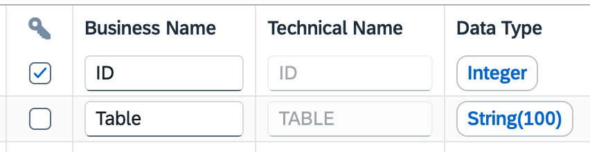
    I also created a control table for all customer exit variables, including an ID and table name.

    Control Table
    Control Table

    Then, I created a master view, or a class, depending on what you would call it. This object determines the corresponding table for the customer exit depending on the ID

    DECLARE lt_result TABLE ("USER" NVARCHAR(100), "VALUE" NVARCHAR(100)); 
    DECLARE lv_table_name NVARCHAR(100);
    
    -- Get Table for determinination
    EXEC 'Select "TABLE" from "TM"."0LT_CUSTOMER_EXITS" WHERE "ID" = ' || :I_VNAM into lv_table_name;
    
    -- Get values for the user
    EXEC 'SELECT "USER", "VALUE" FROM "' || :lv_table_name || '"' INTO lt_result;
    
    
    return SELECT * FROM :lt_result where "USER" = lower(session_context('APPLICATIONUSER'));
    

    The lookup entity for the company code is a new view that calls the central view/class and returns the company codes that I want to use to the variable.

    -- I_VNAM: ID of the entry in the Table 0LT_CUSTOMER_EXITS
    
    select CAST("VALUE" AS VARCHAR(4)) AS COMPANY_CODE from "1SV_CE_DETERMINE_VALUES"(I_VNAM: 1)
    

    This approach allows me to be flexible by determining the corresponding table for the exit centrally and using separate logic for the lookup. I could also build another lookup with a join or
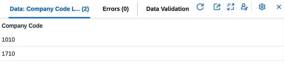
    other filtering options. The preview looks like this:

    Result of data preview
    Result of data preview

    In an SAP Analytics Cloud story, the prompt looks like this:

    SAP Analytics Cloud story prompt
    SAP Analytics Cloud story prompt

    This is an example of how to use derived and dynamic default variables in SAP Datasphere.

    Conclusion

    Let me know in the comments if this approach is something you’re interested in or if you have a completely different approach.

    author.


    Hi,

    I am Tobias, I write this blog since 2014, you can find me on LinkedIn and
    YouTube. I work as a Data &
    Analytics Consultant. If you want, you can leave me a PayPal coffee donation.
    You can also contact me directly if you want.


  • DSAG Meeting about SAP Datasphere

    Yesterday I was at the DSAG TG Datasphere. DSAG is the German SAP user group. The TG Datasphere is a topic group about SAP Datasphere.


    Thanks Hakan for the invitation to the Porsche Campus in Zuffenhausen. It is always great to see the campus and all the nice sports cars.


    But back to the topic. The agenda was packed with lots of slots, including 3 speed dating project experiences. This approach was cool (for the audience, the speaker has to do the presentation 3
    times 😉 ) 


    But the first presentation was by Fabian about the
    SAP Data & Analytics Strategy. Here we heard all about SAP Business Data Cloud (BDC) and the strategy for enterprise data. There was also a detailed answer on how to deal with the old BW in
    the Private Cloud Edition (PCE) and what SAP’s approach is here.

    Then we had the 3 speed dating sessions. One from Sebastian about a Datasphere reference architecture and some project acceleration tools. The next one was a demonstration of
    data products @ Porsche by Hakan. This is also nice,
    but I don’t think many customers are there at the moment. 


    The last one was a presentation about the future architecture @ BAUER. They showed how to implement a business accounting form within SAP Datasphere. Thanks to Andreas and the team for the insight.

    After lunch, Sandy gave us an overview of the best of SAP BW features in SAP
    Datasphere. And also how the SAP Business Warehouse is located in the SAP Business Data Cloud. We saw some features like the devolution of variables with a great example and had the opportunity
    to discuss missing features and ideas. 

    Next was a project experience report from Alena and Anas. They showed how they implemented HR reporting in SAP Datasphere and the challenges they faced

    The last slot was covered by Florian with
    Data Products and what SAP will do in the future. This sounds interesting, but is still far away from the customers.

    Conclusion

    All in all, it was an interesting event. Thanks for the organization and also for the opportunity to see familiar faces and have some good conversations.


    See you next time 

    author.


    Hi,

    I am Tobias, I write this blog since 2014, you can find me on LinkedIn and
    YouTube. I work as a Data &
    Analytics Consultant. If you want, you can leave me a PayPal coffee donation.
    You can also contact me directly if you want.


  • Get all table sizes and records in SAP Datasphere

    If you come from the good old SAP Business Warehouse, you will remember the DB02 transaction. This transaction could show you all the tables in your system and how big they were. I showed an
    example on LinkedIn last year

    DB02 (Screenshot by sapbasisinfo.com)
    DB02 (Screenshot by sapbasisinfo.com)

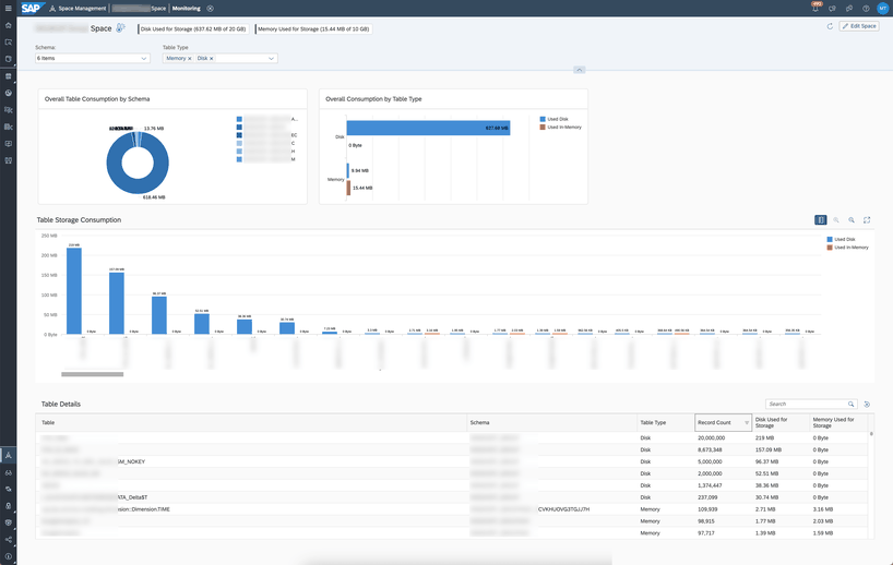
    In SAP Datasphere, you have something similar in the Space Management Monitor. It lists all tables and persistent views with their size and number of records.

    Datasphere: Space Monitor
    Datasphere: Space Monitor

    This is nice, but not ideal, because it is limited to the space you have chosen. I have written a little Python program that shows you all the tables and persistent views in one overview. At the
    moment I always use Excel for the output, but you can modify this line and write it in the terminal or any other application.


    The full source code is available on my GitHub
    repository. But I will explain how it works here. As you know, authentication is moved to a separate class, so I don’t need it in all my programs again.

    Start with the main function.

    if __name__ == "__main__":
        parser = argparse.ArgumentParser(description="Get an overview of all tables over all spaces")
        parser.add_argument("-f", "--file", required=True, help="Path of parameter file")
        args = parser.parse_args()
    
        with open(args.file, 'r') as f:
            config = json.load(f)
    
        secrets_file = config["SETTINGS"]["secrets_file"]
        token_file = config["SETTINGS"]["token_file"]
        dsp_host = config["DATASPHERE"]["dsp_host"]
    
        # Now roll the dice and go to work
        print("Started...")
        get_database_tables()
        print("Ended")
    

    The tool has only one parameter which I use to read a JSON file for all the necessary information like, secret, token, URL and so on. The whole logic is based on my function
    get_database_tables.

    Get Database Tables

    Here you have the OAuth first, and then I read the URL for all the spaces. The URL is https://xyz.eu10.hcs.cloud.sap/dwaas-core/api/v1/spaces

    def get_database_tables():
        header = utils.initializeGetOAuthSession(token_file, secrets_file)
        database_tables = []
    
        url = utils.get_url(dsp_host, 'list_of_spaces')
        response = requests.get(url,headers=header)
        space_list = response.json()
    

    So now I have a list of all the spaces in my tenant and I go through each space with
    this URL https://xyz.eu10.hcs.cloud.sap/dwaas-core/resources/spaces?tables=true&spaceids={spaceID}


    There I have to change the SpaceID with each space, then loop through all the tables of my space and calculate all the key figures like used disk, used memory and records.

        for spaceID in space_list:
            url = utils.get_url(dsp_host, 'space_tables').format(**{"spaceID": spaceID})
            response = requests.get(url, headers=header)
            space_json = response.json()
            try:
                for table in space_json[spaceID]['tables']:
                    tableName = table['tableName']
                    usedDisk = round((table['usedDisk'] / 1000 / 1000),2) # MB
                    usedMemory = round(table['usedMemory'] / 1000 / 1000,2)
                    records = table['recordCount']
                    database_tables.append((spaceID, tableName, usedDisk, usedMemory, records))
            except KeyError:
                continue
    

    Then I publish it in my Excel file.


        df = pd.DataFrame(database_tables, columns=['Space', 'Table Name', 'Used Disk', 'Used Memory', 'Records'])
        df.to_excel(excel_file, sheet_name='Sheet1', index=False)
    

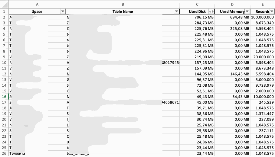
    This is the result: 

    Overview of all tables
    Overview of all tables

    Conclusion

    So now I have all the tables in one place and can see if something is wrong across the tenant. I hope you like this, and if you have any questions, use the comments below. 

    author.


    Hi,

    I am Tobias, I write this blog since 2014, you can find me on LinkedIn and
    YouTube. I work as a Data &
    Analytics Consultant. If you want, you can leave me a PayPal coffee donation.
    You can also contact me directly if you want.


  • Get all exposed views from SAP Datasphere

    Now that we know how to authenticate to the SAP Datasphere API. We can now look at my example that I posted on LinkedIn last year. The goal is to get all the views that are exposed for
    consumption. If you set this flag, you can consume this view with a 3rd party tool such as PowerBi. 


    So if a view is flagged as exposed for consumption, this could be a data leakage issue if there is no Data Access Control (DAC) in place. So I also want to see if a view is exposed
    and if so, if it has a Data Access Control assigned to it. This allows me to identify incorrectly exposed views and see if anyone has access to data without DACs.


    All code examples are available on my GitHub repository


    Every tool has the authentication part, so I moved it to a separate class. If you want to know how to build it, read the last blog post.

    1. Start the program

    So let’s start with the explanation of the program. As I will be using it from the terminal, I want to parametrize it and not have any fixed values inside. To do this, I use the
    ArgumentParser for the config file and the space name I want to check. I read the parameter for all the necessary information like the host, the password and so on from it.

    if __name__ == "__main__":
    
        parser = argparse.ArgumentParser(description="Get all exposed views of a space")
    
        parser.add_argument("-f", "--file", required=True, help="Path of parameter file")
        parser.add_argument("-s", "--space", required=True, help="Space")
    
        args = parser.parse_args()
    
        with open(args.file, 'r') as f:
            config = json.load(f)
    
        dsp_host = config["DATASPHERE"]["dsp_host"]
        dsp_space = args.space
        hdb_address = config["HDB"]["hdb_address"]
        hdb_port = config["HDB"]["hdb_port"]
        hdb_user = config["HDB"]["hdb_user"]
        hdb_password = config["HDB"]["hdb_password"]
    
        # Now roll the dice and go to work
        print("Started...")
        get_exposed_views()
        print("Ended")
    

    I always use this logic, so I don’t have to declare all the information in each tool.  The JSON file I read has the following structure:


    {
      "DATASPHERE": {
        "dsp_host": "https://xyz.eu10.hcs.cloud.sap"
      },
      "HDB": {
        "hdb_address": "xyz.hana.prod-eu10.hanacloud.ondemand.com",
        "hdb_port": 443,
        "hdb_user": "user",
        "hdb_password": "password"
      },
      "SETTINGS": {
        "secrets_file": "secret.json",
        "token_file": "token.json",
        "deploy_wait_time_in_seconds": 0,
        "export_folder_path": "",   
        "view_name_prefix": "1GV",
        "start_technical_name": 7
      }
    }
    

    Get all csn files

    The main function is the get_exposed_views function. There is the logon to the HANA Cloud Database to get the CSN annotations of all objects.


    def get_csn_files():
        # Connect to HDB
        conn = dbapi.connect(
            address=hdb_address,
            port=int(hdb_port),
            user=hdb_user,
            password=hdb_password
        )
        cursor = conn.cursor()
    
        # select statement to fetch csn's. Selection on highest ARTIFACT_VERSION for each object.
        st = f'''
            SELECT A.ARTIFACT_NAME, A.CSN, A.ARTIFACT_VERSION
            FROM "{dsp_space}$TEC"."$$DEPLOY_ARTIFACTS$$" A
            INNER JOIN (
              SELECT ARTIFACT_NAME, MAX(ARTIFACT_VERSION) AS MAX_ARTIFACT_VERSION
              FROM "{dsp_space}$TEC"."$$DEPLOY_ARTIFACTS$$"
              WHERE SCHEMA_NAME = '{dsp_space}' AND ARTIFACT_NAME NOT LIKE '%$%' AND PLUGIN_NAME in ('tableFunction', 'InAModel')
              GROUP BY ARTIFACT_NAME
    
            ) B
            ON A.ARTIFACT_NAME = B.ARTIFACT_NAME
            AND A.ARTIFACT_VERSION = B.MAX_ARTIFACT_VERSION;
        '''
        cursor.execute(st)
        rows = cursor.fetchall()
        conn.close()
        total_rows = len(rows)
        print('Total rows: ' + str(total_rows))
        return rows
    

    As you can see, we are selecting the csn column from the $TEC schema of the previously provided space. And return the rows to the get_exposed_views function.

    Get exposed views

    Once we have all the objects, we can loop through the CSN definitions of the objects. In the CSN annotation, there is a key called „consumption.external“. So we can read this parameter and see if
    a view is exposed or not.


    def get_exposed_views():
        exposedViews = []
        dac_objects = []
        dac_items = []
    
        # Get objects which are exposed
        csn_files = get_csn_files()
    
        for csn in csn_files:
            csn = csn[1]
            csn_loaded = json.loads(csn)
            dac_objects.clear()
            dac_items.clear()
    
            objectName = list(csn_loaded['definitions'].keys())[0]
            label = csn_loaded['definitions'][objectName]['@EndUserText.label']
            try:
                exposed = csn_loaded['definitions'][objectName]['@DataWarehouse.consumption.external']
            except KeyError:
                exposed = False
    

    The next check is to see if the object has a Data Access Control (DAC) assigned to it. For this we have the key „dataAccessControl.usage“ which shows the information. 


            try:
                for dac in csn_loaded['definitions'][objectName]['@DataWarehouse.dataAccessControl.usage']:
    
                    if len(dac['on']) == 3: # one column mapping
                        dac_items.append(dac['on'][0]['ref'][0])
    
                    if len(dac['on']) == 7: # two column mapping
                        dac_items.append(dac['on'][0]['ref'][0])
                        dac_items.append(dac['on'][4]['ref'][0])
    
                    dac_objects.append(dac["target"])
    
            except KeyError:
                dac_items.clear()
                dac_objects.clear()
    

    At the end I create a list which I publish via a Pandas data frame to Excel and format this Excel in the right way.


            exposedViews.append((dsp_space, objectName, label, exposed, ', '.join(f'{item}' for item in dac_items), ', '.join(f'{object}' for object in dac_objects)))
    
        df = pd.DataFrame(exposedViews, columns=['Space', 'Object', 'Description', 'Exposed', 'DAC Item', 'DAC Object'])
        df.to_excel(excel_file, sheet_name='Sheet1', index=False)
    
        # Format Excel
        utils.format_excel(excel_file)
    

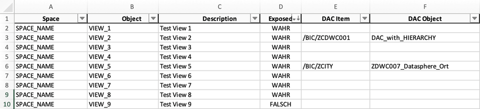
    Output

    Output of all exposed views in Excel
    Output of all exposed views in Excel

    Conclusion

    This is the magic to get all the views that are exposed and have a data access control assigned or not. This is the first of many ideas I would like to share with you using the Datasphere
    API and HANA Cloud Database. 


    Thanks again to Andreas Dietz for the initial idea. Please share your thoughts in the comments.

    author.

    Hi,

    I am Tobias, I write this blog since 2014, you can find me on LinkedIn and
    YouTube. I work as a Data &
    Analytics Consultant. If you want, you can leave me a PayPal coffee donation.
    You can also contact me directly if you want.


  • SAP Datasphere API and Python Authentication

    Now that we know how to get data from the SAP Datasphere API using Postman, I want to automate the steps using Python. In this post, I implement authentication via OAuth. I use the two
    existing libraries OAuth2Session and urllib.parse. 


    To create the OAuth request we need the secret, the client ID, the authorization URL and the token URL. I stored all this information in a JSON file so I can read and process it. Where to get
    this information can be found in the earlier post. So we need to read the JSON file first to
    get all the parameters.


    secrets_file = path_to_the_secret.json
    
    f = open(secrets_file)
    secrets = json.load(f)
    print(secrets)


    Next, we need to encode the client ID, as described by Jascha in this post. I use the
    urllib.parse.quote functionality for this..

    client_id_encode = urllib.parse.quote(secrets['client_id'])
    

    With the print command, you should see a result like this: sb-e4c75210-40c4-4c89-a960-381b156c4e93%21b106441%7Cclient%21b3650


    Once we have the encoded client ID, we can create the URL for authentication. For this, we need the authorization URL and combine it with the client ID. 


    code_url = secrets['authorization_url'] + '?response_type=code&client_id=' + client_id_encode 


    When you print the URL, it should look like this:

    https://xyz.authentication.eu10.hana.ondemand.com/oauth/authorize?response_type=code&client_id=sb-e4c75210-40c4-4c89-a960-381b156c4e93%21b106441%7Cclient%21b3650

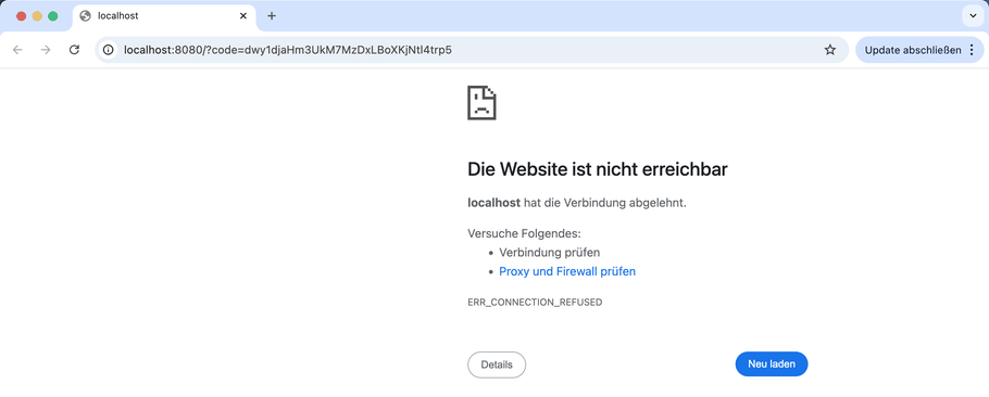
    Open the printed URL in a browser and copy the code you get at the end. 

    Receive code after authentication
    Receive code after authentication

    Now we can create the session object for the request.

    session = requests.session() 


    And use an input function to store the code we get from the above url, see screenshot

    Enter code in Python program
    Enter code in Python program

    This is all we need for the OAuth process with Python.

    OAuth_AccessRequest = session.post( secrets['token_url'],
                                        auth=(secrets['client_id'], secrets['client_secret']),
                                        headers={"x-sap-sac-custom-auth": "true",
                                                 "content-type": "application/x-www-form-urlencoded",
                                                 "redirect_uri": 'http://localhost'
                                                },
                                        data={'grant_type': 'authorization_code',
                                              'code': code,
                                              'response_type': 'token'
                                             }
                                      )
    

    As you can see, we use the token URL, the client ID, the client secret, and the code we got from the URL earlier. The redirect is localhost, where we added the OAuth client. With the print
    statement, we can print the JSON response from the request.


    print(OAuth_AccessRequest.json())
    
    Obtain an OAuth access token for later use
    Obtain an OAuth access token for later use

    That is all the magic. We are now using Python to authenticate to the SAP Datasphere API. The next steps are to store the information for future use and to renew the token when it expires.
    In my example, I store the information in a file and use it to renew the token. 


    token = OAuth_AccessRequest.json()
    with open(path, 'w') as f:
       json.dump(token, f)


    Updating the token is simple. First, we need to read the file where we previously stored the information. Open the file with the secret information, create an OAuth session object, and refresh
    the token.


    f = open(token_file)
    token = json.load(f)
    
    f = open(path_of_secret_file)
    secrets = json.load(f)
    
    extra = { 'client_id': secrets['client_id'],
              'client_secret': secrets['client_secret']
            }
    
    datasphere = OAuth2Session(secrets['client_id'], token=token)
    token = datasphere.refresh_token(token_url=secrets['token_url'], **extra)
    

    Conclusion

    That’s it. You can now authenticate to the Datasphere API using OAuth from Python. I know there’s a manual step in the code, but that’s not a showstopper for me right now. I only need to
    authenticate with the code after 30 days, and that is fine for some admin tools. If you want to automate some data extractions, then you can build something for that. Jascha described a way in
    this post. I look forward to hearing from you
    and your ideas about what we can do with Python and the API in the future. The next blog will be about processing information with Python, so stay tuned.

    author.

    Hi,

    I am Tobias, I write this blog since 2014, you can find me on LinkedIn and
    YouTube. I work as a Data &
    Analytics Consultant. If you want, you can leave me a PayPal coffee donation.
    You can also contact me directly if you want.


  • Deeper Look into SAP Datasphere API

    Now that we know how to use Postman to send an API request to SAP Datasphere and receive data. We
    can now take a closer look at the API and what we can do with it. At api.sap.com we get different API
    endpoints, I want to focus on the consumption part. The API reference for the consumption part allows us to consume relational and analytical models. 


    Let’s start with the relational models and retrieve the data with Postman to see some results. The relational API endpoint can be accessed at this URL


    https://xyz.eu10.hcs.cloud.sap/api/v1/dwc/consumption/relational/{space}/{asset}/{technical_object}


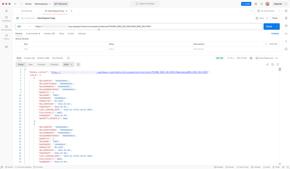
    You can find the exact description in the API catalog. So I won’t copy and paste the content here.  Now let’s get the data with the above URL. My view is called DBV_BIKE_DELIVERY.
    If I now use my OAuth from the last post, I get the data directly in Postman.

    Get data from relational view with Postman
    Get data from relational view with Postman

    As you can see, it is very easy to retrieve the data from the API. To make it more flexible, the URL can have different parameters like

    • select
    • filter
    • order by
    • top
    • skip

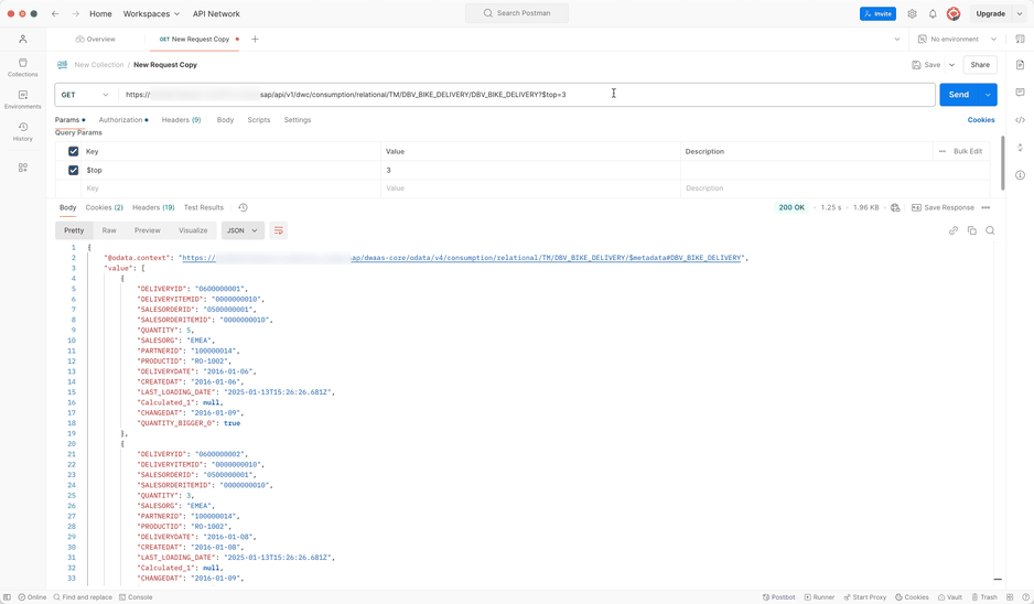
    This can be really interesting when we use this URL later with Python to get more flexible data. For example, if we use the $top parameter, we can display only the top 3 records.

    Get top 3 entries of relational view
    Get top 3 entries of relational view

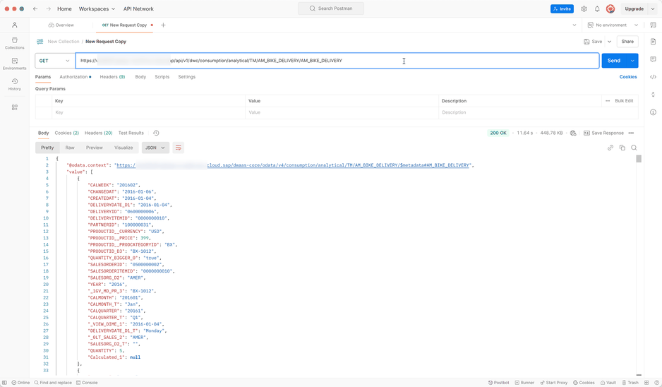
    Now you can use Postman to access relational views and retrieve the data. The next step is to retrieve data from analytical objects such as an analytical model. The URL is almost the same:


    https://xyz.eu10.hcs.cloud.sap/api/v1/dwc/consumption/analytical/{space}/{asset}/{technical_object}


    As you can see, the only difference is the word relational to analytical. 

    Get data from analytic model
    Get data from analytic model

    With the analytic URL, we get data from an analytic model. The advantage of the analytic model is that we also get data from associated dimensions in the result. So the result can be very large
    because all active dimension attributes are now displayed. So be careful what you select.


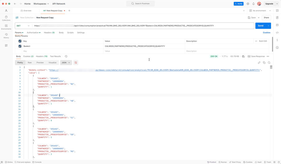
    To reduce the dimensions you want to consume, we can add the parameter $select and get only the columns we need.

    Get specific columns from analytic model
    Get specific columns from analytic model

    So now we only get the 4 columns I added to the URL. The columns are 

    • CALWEEK
    • PARTNERID
    • PRODUCTID__PRODCATEGORYID
    • QUANTITY

    As you can see, I get different columns. The CALWEEK column from the associated time dimension, the PARTNERID and Quantity from the fact view, and the PRODUCTCATEGORYID from the product
    dimension. 


    I think this offers a lot of possibilities for getting data out of Datasphere.

    Conclusion

    In this post, I looked deeper into the SAP Datasphere API to get data directly from the system. You can access relational views or analytical models and consume them in other tools. Prerequisite
    is the OAuth we created in the previous post. What do you think about accessing the data via API? 


    In the next post we will switch to Python and try to get the data we have consumed with post in Python. 

    author.


    Hi,

    I am Tobias, I write this blog since 2014, you can find me on Twitter,
    Facebook and YouTube. I work as a Senior Business
    Warehouse Consultant. In 2016, I wrote the first edition of . If you want, you can leave me a PayPal coffee donation.
    You can also contact me directly if you want.


  • Create API requests in SAP Datasphere with Postman

    This is the first in a series of articles about the SAP Datasphere API and what you can do with it. I will start by explaining how to configure the OAuth and start with the first request
    using Postman. Postman is a tool for creating requests to web services. 


    So let’s dive into it. If you want to consume the SAP Datasphere API, you need to find the right endpoints. A good place to start is api.sap.com. But how can we test and see if the request is correct? If we get the right result?


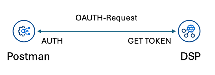
    In this post, I will go through the configuration of Postman that allows you to send requests and also receive data from those requests. To do this, we use OAuth technology. I won’t explain what
    OAuth is. If you are interested, take a look at Wikipedia


    Basic OAuth logic
    Basic OAuth logic

    First, we need an OAuth connection. To create an OAuth connection, go to your SAP Datasphere tenant and select System >> Administration >> APP Integration. There you will
    find the authorization and token URL that you will need to create a token later.

    OAuth URLs
    OAuth URLs

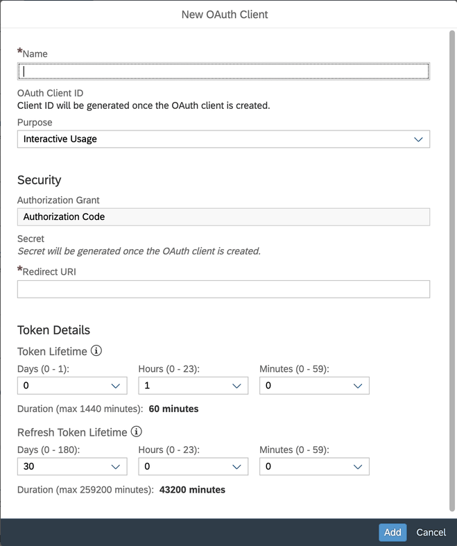
    Now we need to create a client so we have a client id and a secret id. Click Create New OAuth Client.

    Create a new OAuth client
    Create a new OAuth client

    Define a name, the purpose, a redirect URL (in this case http://localhost:8080), and as of release 2024.8 you can also define some details about the token. After clicking add, the new OAuth
    client is created. Now we need the secret and the client id for authorization. Copy the OAuth client ID and secret for later use. 


    Now we have everything we need to access the API. Let’s switch to Postman, you can use it either on the web or via the downloaded program. Visit https://www.postman.com for more information.

    Create a new request in Postman
    Create a new request in Postman

    Go to the Authorization tab, select the OAuth 2.0 type, and select Request Headers for the „Add the authorization information to“ section. Now we need to add the token
    information.  


    • Use token type: Access Token
    • Header Prefix: Bearer
    • Auto-refresh token: True
    • Grant type: Authorization Code
    • Callback URL: http://localhost:8080
    • Auth URL: Auth URL from the Datasphere tenant (e.g. https://xyz.authentication.eu10.hana.ondemand.com/oauth/authorize)
    • Access Token URL: Token URL from the tenant (e.g. https://xyz.authentication.eu10.hana.ondemand.com/oauth/token)
    • Client ID: Client ID from the OAuth we created earlier
    • Client secret: Client Secret we get earlier from the OAuth.
    • Client authentication: Send as Basic Auth header

    Click „Get New Access Token“ to create a new token. This will take you to your SAP Datasphere login page, where you will need to log in for the first time. You will receive the token
    and can use it. 


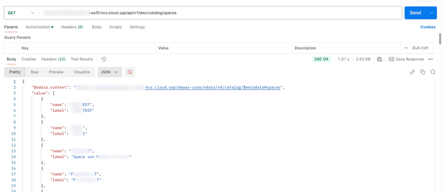
    Now we are ready to kick against the Datasphere API and get some results. To give you a first look at the API, we use the following URL
    https://xyz.eu10.hcs.cloud.sap/api/v1/dwc/catalog/spaces to get a result of all the spaces. As you can see in the screenshot below, the http status is 200. This means that
    the request was successful.


    The next post will go deeper into the API endpoints and some use cases.

    Result of SAP Datasphere API
    Result of SAP Datasphere API

    Conclusion

    This is the first of a series of posts about the SAP Datasphere API. I hope you now understand the basics and how to check if your requests return data or if something went wrong. There is also
    an old post in the SAP community about Postman configuration. But as
    far as I know, sometimes SAP deletes all the old stuff, and you cannot find it anymore. So feel free to use the comments and give me some ideas what I should show with the API in the next posts.

    author.

    Hi,

    I am Tobias, I write this blog since 2014, you can find me on LinkedIn and
    YouTube. I work as a Data &
    Analytics Consultant. If you want, you can leave me a PayPal coffee donation.
    You can also contact me directly if you want.


  • Dynamic filter push down in SAP Datasphere

    Dynamic source filtering is a big issue in SAP Datasphere. There are several approaches that may work for one, but not for another. 

     

    The discussion started again on LinkedIn after I read a post about dynamic filtering that was set with a fixed filter. Wanda then showed us a solution he uses to filter
    data. But
    Christopher
    pointed out that the filter is not pushed down to the source when you use a DP agent, e.g., the ABAP connection.


    I had in mind that there was a blog post about how to push a filter down, even on an ABAP connection. So I tried Wanda’s idea and combined it with the other knowledge. This blog post will show
    you how it works.


    If you already know s-note 2567999, you know that you can filter data with a stored
    procedure. And as of June, you can run stored procedures directly in task chains. This is a really nice feature. But back to the other solution.


    First, we need a local table to store the load parameter for this approach. The loading table is just to set the parameter easily and not always in the coding.


    It is quite simple. 3 columns, one for the application, one for the parameter and one for the value. It may be different on your approach, but keep in mind to adjust the coding as well.

    Structure of loading table in SAP Datasphere
    Structure of loading table in SAP Datasphere

    On the local table, we now need a SQL script view with the logic. The coding is simple, as Wanda described in his LinkedIn post.


    return
    select 
        case 
            when APP_NAME = 'APP_1' AND PARAM_NAME = 'TEST' then
                case
                    when PARAM_VALUE is null then
                        add_days(to_date(now()), -1)
                    else
                        to_date(PARAM_VALUE)
                end
            else
                to_date(now())
        END as PARAM_VALUE
        
    from "0LT_LOADING_PARAMETER"
    where
    APP_NAME = :I_APP_NAME
    and PARAM_NAME = :I_PARAM_NAME;
    

    We have one return parameter (PARAM_VALUE) and two input parameters (I_APP_NAME and I_PARAM_NAME). That was it. Now the magic needs to be done in a new SQL script view. Based on this
    post. I tried to combine the logic from Wanda with this approach to
    push the filter down on a SAP BW Connection. The logic in this example is quite simple.


    DECLARE myDate DATE;
    DECLARE myDateString NVARCHAR(8);
    
    select PARAM_VALUE into myDate from "1SV_FUNCTION_PARAMETER"(I_APP_NAME=>'APP_1',I_PARAM_NAME=>'TEST');
    
    myDateString = TO_NVARCHAR(myDate, 'YYYYMMDD');
    
    return select "RECORDMODE","ORT","ARTIKEL","DATE1","QUANTITY" from "ZDWC003" where "DATE1" = myDateString;


    What we do is get the date from the function parameter (see above) and convert it to the correct format for the connection date (in this case, YYYYMMDD). Then we display the result.

    SAP Datasphere connection overview
    SAP Datasphere connection overview
    Push down works, see where statement
    Push down works, see where statement
    Result preview of remote table to see the amount of entries match
    Result preview of remote table to see the amount of entries match

    As you can see, the filter is pushed down when the condition is equal. If I use >= then the filter is not pushed down.

    Push down failed
    Push down failed

    Conclusion

    You can see it in the WHERE clause. I hope this helps you a bit and gives you an option how to solve your problem with dynamic filtering. I hope we get a good solution directly from SAP because
    this is not a small problem. The same should work for replication flows. 


    The filter push down is necessary for old SAP systems and also for non-SAP systems. We will see what comes in 2025. 

    author.


    Hi,

    I am Tobias, I write this blog since 2014, you can find me on LinkedIn and
    YouTube. I work as a Data &
    Analytics Consultant. If you want, you can leave me a PayPal coffee donation.
    You can also contact me directly if you want.